Conventions¶

Units¶

Angles are expressed in degrees, while all other units in the dataset use the International System (SI), such as meters and seconds, unless otherwise indicated by a "unit" key. For example, the Bitfield and Percent units are used for datasets in the file.

Quantity	Symbol, usual script (common)	Units
Distance, positions	X, Y, Z	meter [m]
Time	t	second [s]
Mass	M	kilogram [kg]
Speed	c	[m/s]
Angle	α, β, γ, θ, φ	degree [°]
Density	ρ	[kg/m³]
Gain	G	dB

Axes and coordinate systems¶

The following coordinate systems are defined and used for storing and locating the position of each element in space. A transformation, such as through the use of homogeneous coordinates and transformation matrices, can be defined between each coordinate systems using the parameters stored in the Setup JSON formatted dataset.

Global referential coordinate system¶

\((X,Y,Z)\)

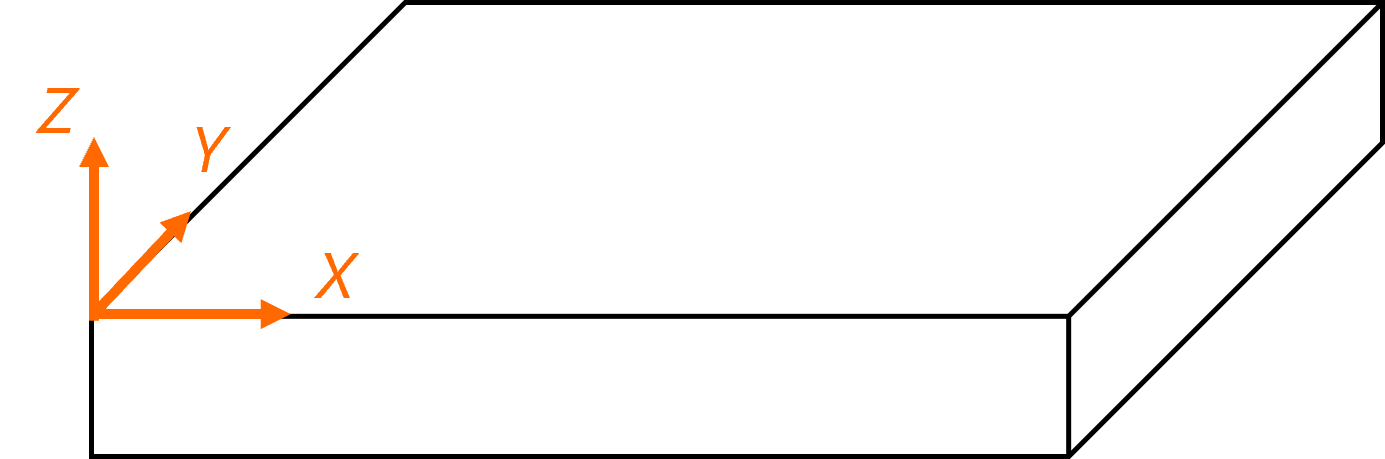
It is independent of the acquisition and serves to position the data on the specimen in the real world.
Origin and orientation: Arbitrary and stays the same across files for a given specimen. It is usually defined by the user on the specimen with some marking or physical reference in the specimen environment.

NOTE: Currently, the \(X\), \(Y\), and \(Z\) axes are not used nor defined in the NDE file, but to show inspection results in 3D, one would have to translate everything to this coordinate system.

Specimen surface coordinate system¶

\((U,V,W)\)

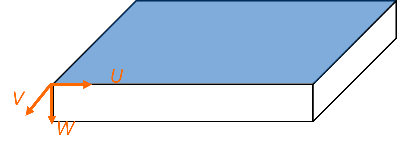
In scenarios where probe positioning is in direct relation to the surface, the position on the surface of a specimen, \((X, Y, Z)\) in global coordinates, is transformed into \((U,V)\) surface-orthogonal curvilinear coordinates. Take note that depending on the scenario, \((U,V)\) may be directly in distance units (meter), but this is not systematic.

To the \((U,V)\) surface mapping coordinates, a depth axis \(W\) is added. The depth \(W\) is defined as being normal to the local \((U,V)\) coordinates and follows the right-hand rule for sign definition, resulting in a \((U,V,W)\) coordinate system.

The \(W\) axis is normal to the surface and always points inside the material.
The \(U\) axis is defined relative to the specimen's feature (per scenario). Its orientation is arbitrary.
The \(V\) axis is perpendicular to \(U\) and its orientation can be inferred with the right-hand rule from the cross product of \(U\) and \(W\).

Local coordinate system¶

\((u,v,w)\)

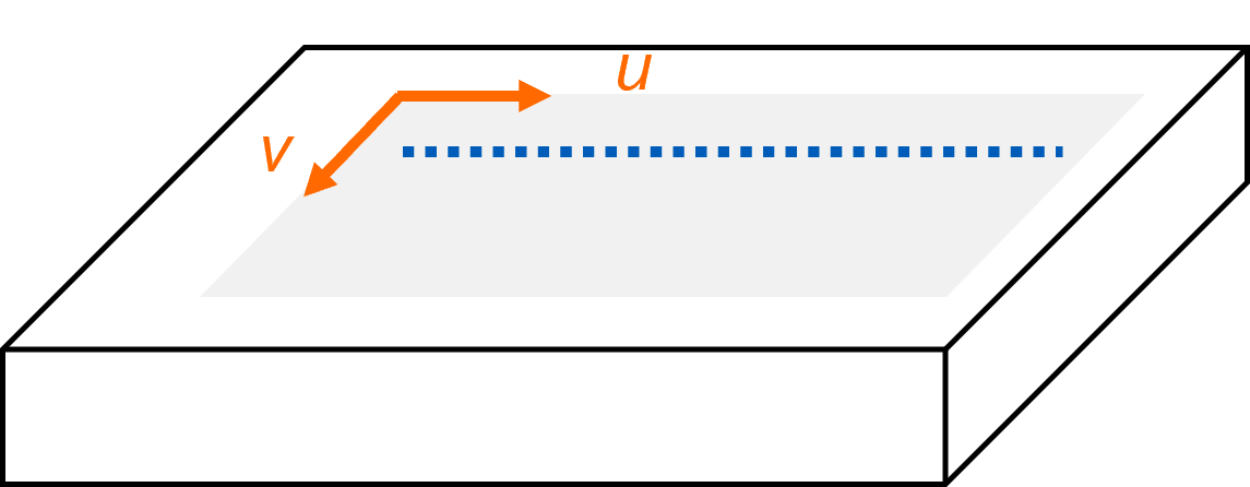
A local coordinate system \((u,v)\) is associated with each scanned area on the specimen surface \((U,V)\). Additionally, the use of \((u,v)\) coordinates is enforced as a way to disambiguate the notions of “scan axis” and “index axis,” which are interpreted depending on the scenario.

The path mechanically followed at the surface of the specimen by the scanner can be referenced in the local coordinate system for simple paths such as one-line and raster scanning.
The local \((u,v)\) curvilinear coordinates (not necessarily in distance units) are linked to the position encoders (in distance units).
The parameter \(u\) is often along the continuous scanning axis, while the \(v\) parameter describes the orthogonal direction.
The parameter \(w\) is along the specimen's local normal.
Multiple wedges coordinate systems \((x_w, y_w, z_w)\) attached to a scanner can be defined using the appropriate offsets with respect to the local frame.

Wedge coordinate system¶

\((x_w, y_w, z_w)\)

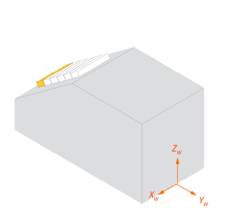
The wedge coordinate system \((x_w, y_w, z_w)\) is typically positioned directly on the surface \((U,V)\) through the local frame \((u,v)\), and thus links the probe position to the specimen.
Origin and orientation: See appropriate wedge object conventions with the appropriate technology (e.g. UT/PAUT, ET) for details.

NOTE: The term wedge is used to describe any device that maintain constant positioning of a probe relative to an inspected surface.

Mounting location coordinate system¶

UT

\((x_m, y_m, z_m)\)

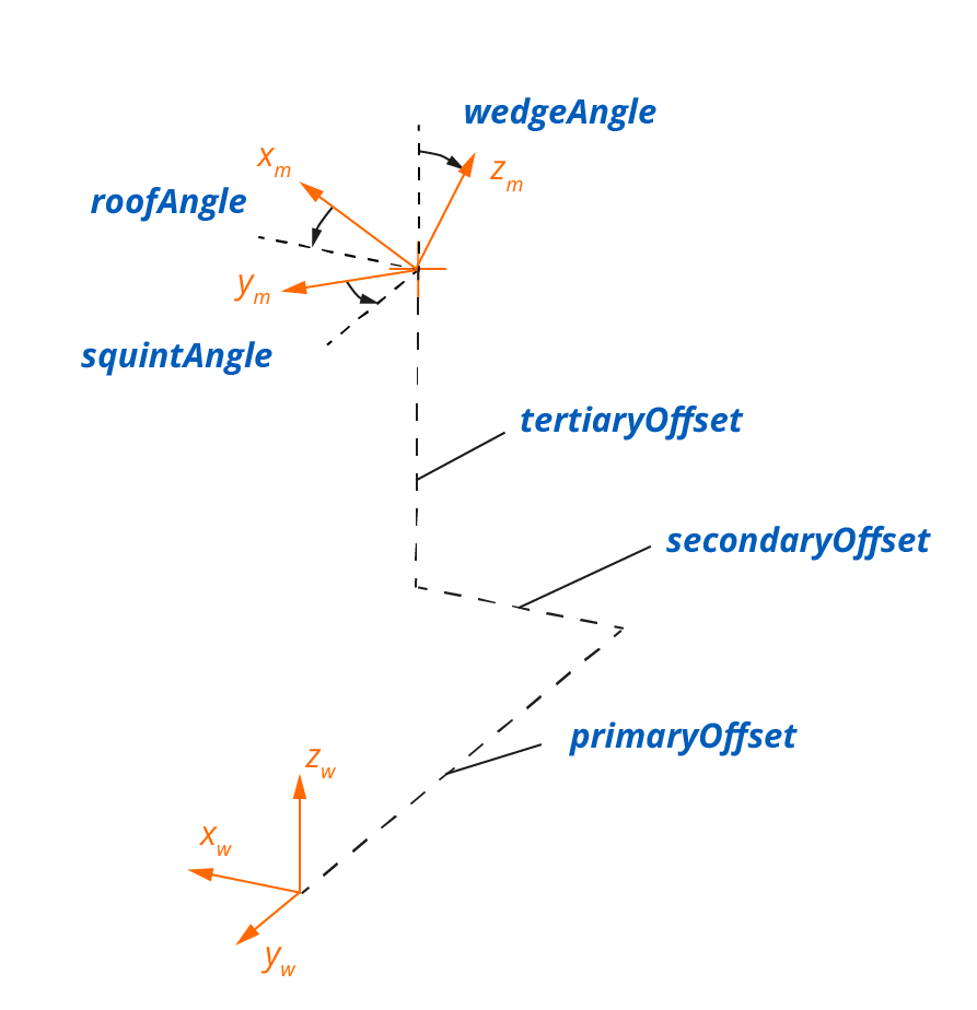
A mounting location coordinate system \((x_m, y_m, z_m)\) is positioned from the wedge reference frame using three offsets (primaryOffset, secondaryOffset and tertiaryOffset) and three angles (wedgeAngle, squintAngle and roofAngle). See the mountingLocations section for more information.

Probe coordinate system¶

The probe coordinate system defines how elements or sensors are positioned relative to the probe body. Its definition differs between technologies.

UT \((x_p, y_p, z_p)\)

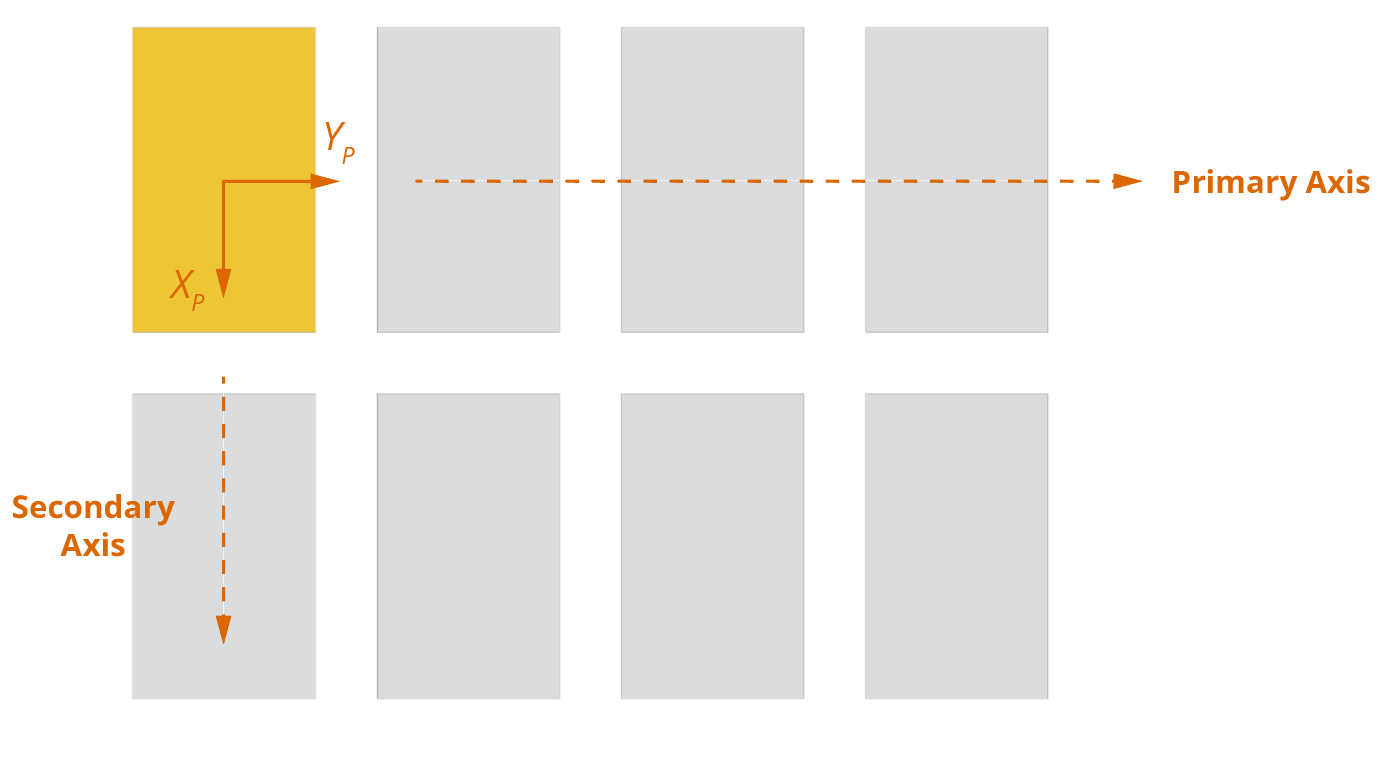
The origin of and ultrasonic probe coordinate system \((x_p, y_p, z_p)\) corresponds to the center of the first element. The probe Primary Axis is along \(y_p\) and the probe Secondary Axis is along \(x_p\). See the phasedArrayLinear probe type for details.

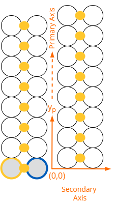
ET \((x_p, y_p, z_p)\)

Eddy current sensors are positioned in a 2D coordinate system co-planar with the specimen surface. The \((0,0)\) origin of the probe coordinate system \((x_p, y_p, z_p)\) is shared across all sensor groups within a probe, and is arbitrary in the file — in practice it typically aligns with a reference marking on the probe body. See the eddyCurrentProbe probe type for details.

Other axes¶

These axes are used in the HDF5 dataset structure rather than as physical coordinate axes.

Encoding axis:

Relates to encoder displacement; coupling to specimen and/or global coordinates is scenario-dependent. Applies to all modalities.

Beams axis: UT

An axis where each element contains one beam's incidence position on the specimen. Used in PAUT scenarios when the beams do not fit well in a \(U\), \(V\) grid, simplifying their use in those scenarios.

Ultrasound axis: UT

Time-based information sampled by an ultrasonic acquisition system. Positioning in global coordinates requires accounting for ray tracing and part velocities.

Channel axis: ET

Identifies each eddy current channel (combination of sensor and inspection parameters) within the dataset.

AcquisitionCycle axis: ET

Sequential index of acquisition cycles recorded by the instrument, used in allCycle data mappings before spatial remapping.

Storage mode¶

Note

The storage mode convention described below applies to discreteGrid data mappings. For Eddy Current acquisitions, raw data is typically stored using an allCycle data mapping instead, which has no storageMode concept.

There are two distinct ways to work with discreteGrid when storing a given dataset.

storageMode: "Independent" is used to store the complete data acquisition sequence in reference to a \((u,0)\) trajectory. For example, a scanner holding multiple PAUT probes with each individually offset relative to the \((u,v)\) reference system could all relate to the same discreteGrid with independent storage mode. In this case, the positioning of the data on or in the specimen requires some processing of individual beams or sensors positions.

storageMode: "Paintbrush" is used to store individual beams or sensor information directly on the corresponding \((u,v)\) position. Practically, Paintbrush is only possible under some hypotheses:

All beams or sensors operates under the same condition. For example, paint brush is possible with linear pulse-echo PAUT but is not possible with sectorial pulse-echo PAUT.
All beams or sensors can be associated with a surface position. For example, FMC acquisition can't be stored as Paintbrush because individual A-scans of the FMC don't have defined surface positioning.
Beams or sensors surface positioning should fit perfectly on the underlying coordinate system grid. Accordingly, the discreteGrid coordinate system grid typically has to be created according to a probe and scanning system characteristic for a Paintbrush storage.

The main advantage of Paintbrush storage is that data is natively mapped on a specimen surface.

UT/PAUT conventions¶

General concepts and hypothesis¶

Material is considered linear, homogeneous, and isotropic by default.
Coupling layers are incapable of transmitting shear waves by default.
A probe has a single nominal center frequency by default.