Example Files
Ultrasonic Testing Examples
General weld scenario
Manual weld scanning using conventional ultrasonic testing (UT)
In this example, a weld bead on a 11 mm thick stainless steel plate is manually scanned using a C540 2.25 MHz single-element angle beam transducer mounted on a ABSA-5T-45 45° wedge. The transducer's position is recorded using a wheel encoder.
UT Weld_Plate_UT-sk90-4.2.nde | Download | View
Manual weld scanning using parallel time-of-flight diffraction (TOFD)
In this example, a 10 mm thick steel pipe comprising a girth weld is manually scanned using a pair of C563 10 MHz single-element angle beam transducers mounted on ST1-70L 70° wedges. The scanning direction is perpendicular to the weld bevel (and parallel to the direction of the beam). The transducer's position is recorded using a wire encoder.
UT Weld_Plate_ToFD_Parallel-4.2.nde | Download | View
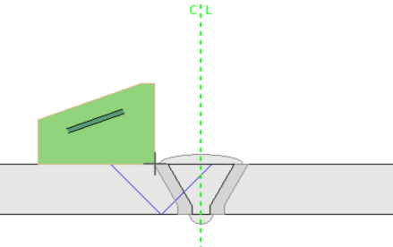
Manual weld scanning using phased array ultrasonic testing (PAUT)
In this first example, a weld bead on a 26 mm thick stainless steel plate is manually scanned using a 5L64-A32 5 MHz 64-element probe mounted on a SA32-N55S 36° wedge. The probe's position is recorded using a wire encoder. This example comprises a conventional sectorial scan with one group.
UT Weld_Plate_PA-Sect_sk90-4.2.nde | Download | View
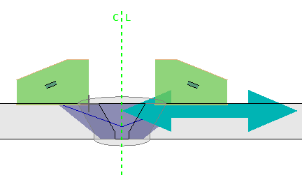
In this second example, a weld bead on a 12.5 mm thick stainless steel plate is manually scanned using a 5L64-A32 5 MHz 64-element probe mounted on a SA32-N55S 36° wedge. The probe's position is recorded using a wire encoder. This example comprises a compound sectorial scan with two groups (8 and 16 elements).
UT Weld_Plate_PA-Comp_sk90-2gr-4.2.nde | Download | View
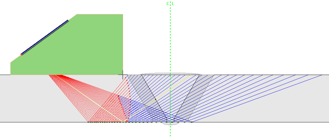
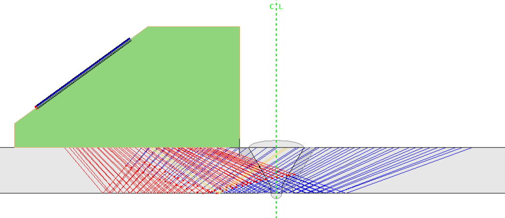
Manual weld scanning using the total focusing method (TFM)
In this example, a weld bead on a 12.5 mm thick stainless steel plate is manually scanned using a 5L64-A32 5 MHz 64-element probe mounted on a SA32-N55S 36° wedge. The probe's position is recorded using a wire encoder. Two group configurations are provided.
Four TFM wavesets/groups: T-T, TT-T, TT-TT, TT-TTT:
UT Weld_Plate_4TFM_sk90-4.2.nde | Download | View
One PCI waveset/group: T-T:
UT Weld_Plate_PCI_sk90-4.2.nde | Download | View
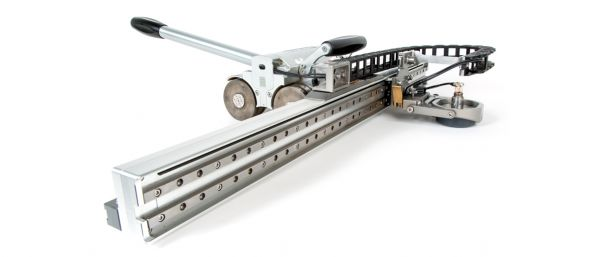
Semiautomated weld scanning using time-of-flight diffraction (TOFD) and phased array ultrasonic testing (PAUT)
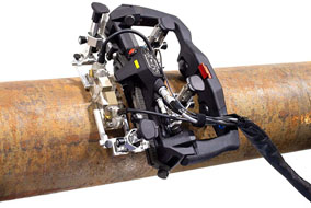
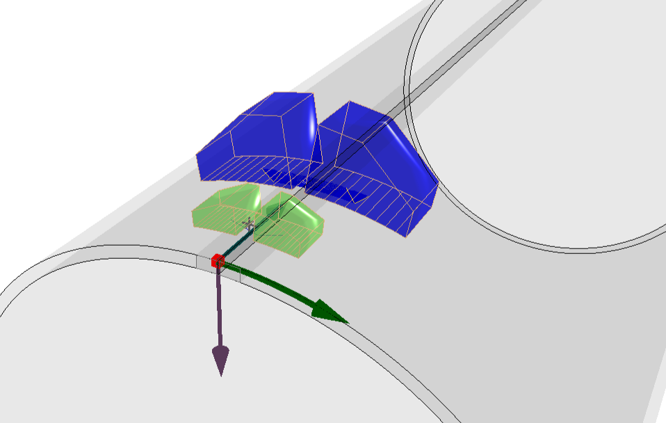
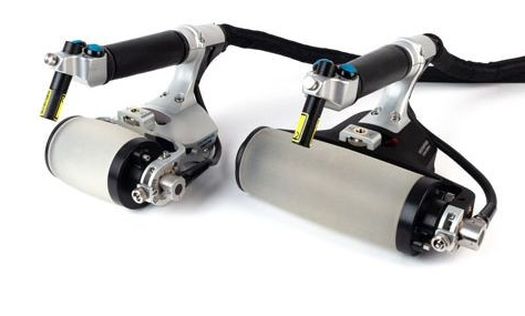
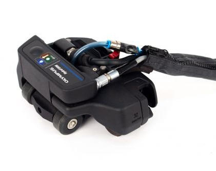
In this example, a 6.15 mm thick steel pipe comprising a longitudinal weld is scanned using the AxSEAM scanner and a pair of C563 10 MHz probes mounted on ST1-70L-IHC 70° wedges for TOFD and a pair of 5L32-A31 5 MHz 32-element probes mounted on SA31-N55S 36° wedges. The probe position is recorded using the scanner encoder.
UT Weld_COD_2PA-ToFD-4.2.nde | Download | View
Semiautomated weld raster scanning using phased array ultrasonic testing (PAUT)
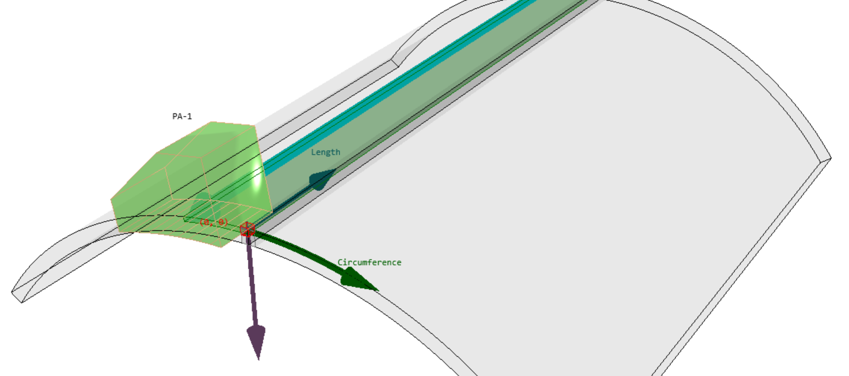
In this example, a 6.35 mm thick steel pipe comprising a longitudinal weld is scanned using the AxSEAM scanner and a 5L32-A31 5 MHz 64-element probe mounted on a SA31-N55S 36° wedge. The probe position is recorded using the scanner encoder.
UT Weld_COD_PA-Raster-4.2.nde | Download | View
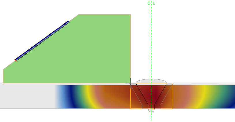
Girth weld scanning using the total focusing method (TFM)
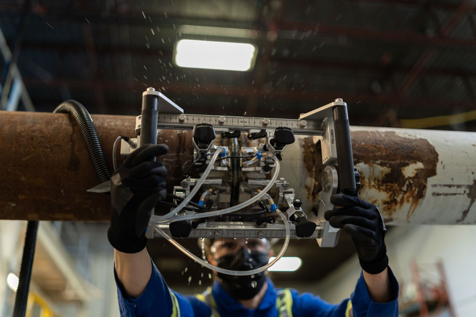
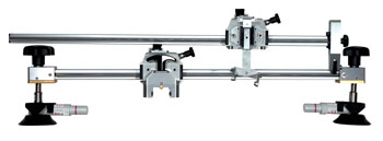
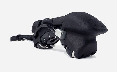
In this example, a 9.5 mm thick steel pipe comprising a circumferential weld is scanned using the HSMT-Flex scanner and a pair of 5L32-A31 5 MHz 32-element probes mounted on SA31-N55S 36° wedges. TFM is performed simultaneously from both sides of the weld bead. The probe position is recorded using the scanner encoder. A post-acquisition analysis was also performed on this file, adding gain to the data.
UT Weld_AOD_DualTFM-Analysis-4.2.nde | Download | View
General mapping scenario
Corrosion inspection using conventional ultrasonic testing (UT)
In this example, a 5.47 mm thick steel pipe is scanned using the MapROVER scanner and a D790 5 MHz dual element transducer. The probe's position is recorded using the scanner encoders.
UT Corr_COD_UT-Raster-4.2.nde | Download | View
Composite wheel probe scanning using phased array ultrasonic testing (PAUT)
In this example, a 10 mm thick plexiglass plate engraved with letters is scanned using the RollerFORM scanner and a 3.5L64-IWP1 3.5 MHz 64-element probe, mimicking the inspection of a carbon fiber reinforced polymer (CFRP) plate. The probe position is recorded using the scanner encoder. A post-acquisition analysis was also performed on this file, adding gain to the data.
Using PAUT:
UT CFRP_Plate_PA-Lin0_sk90-Analysis-4.2.nde | Download | View
Composite X-Y scanning using the total focusing method (TFM)
In this example, a 10 mm thick plexiglass plate engraved with letters is scanned using the Glider scanner and a 5L64-NW1 5 MHz 64-element probe mounted on a SNW1-0L 0° wedge, mimicking the inspection of a carbon fiber reinforced polymer (CFRP) plate. The probe position is recorded using the scanner encoder. Two group configurations are provided.
Using TFM:
UT CFRP_Plate_TFM-Raster_sk90-4.2.nde | Download | View
Using phase coherence imaging (PCI):
UT CFRP_Plate_PCI-Raster_sk90-4.2.nde | Download | View
Corrosion inspection using phased array ultrasonic testing (PAUT)
In this example, a 9.5 mm thick steel plate is scanned using the HydroFORM scanner and a 7.5L64-I8 7.5 MHz 64-element probe. The probe's position is recorded using the scanner encoder.
UT Corr_Plate_PA-Lin0_sk270-4.2.nde | Download | View
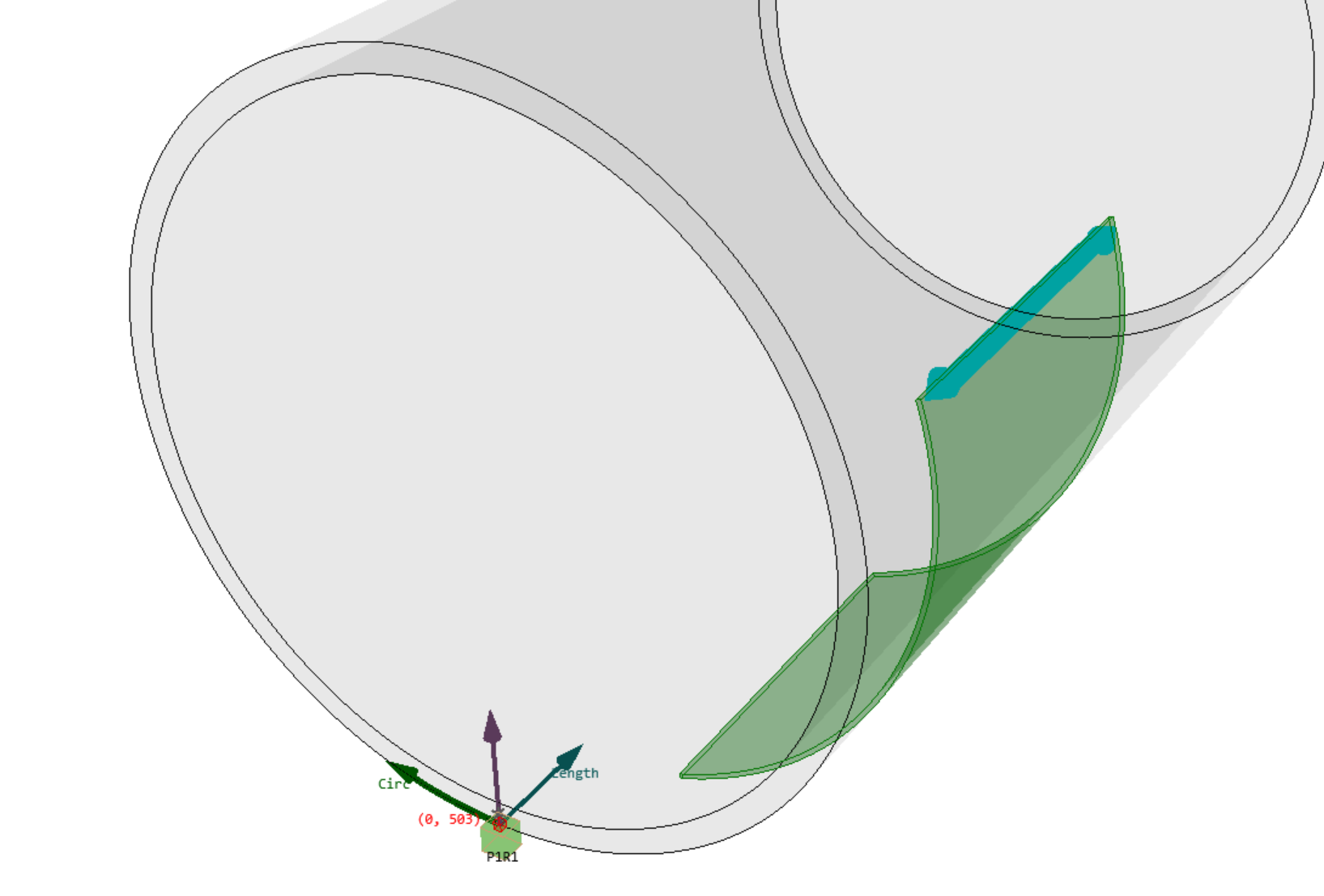
Pipe elbow corrosion inspection using phased array ultrasonic testing (PAUT)
In this example, a 5.5 mm thick elbow pipe is scanned using the FlexoFORM scanner and a 7.5L64-FA1 7.5 MHz 64-element probe. The probe's position is recorded using the scanner encoder. Note that in this case a plate geometry is used, as each element of the probe is maintained normal to the pipe surface for each scanner position. A post-acquisition analysis was also performed on this file, adding gain to the data.
UT Corr_COD_PA-Lin0_sk90-Analysis-4.2.nde | Download | View
Full matrix capture (FMC) acquisition
In this example, a 7.5L60-PWZ1 7.5 MHz 60-element probe is positioned in contact with a steel block containing side-drilled holes. The probe's position is fixed. A single FMC is collected.
Eddy Current Testing Examples
General mapping scenario
Manual Surface Crack Inspection
High-frequency surface crack detection at 1 MHz using a low-pass filter with a cut-off frequency of 300 Hz. The acquisition is time-based.
ET Surface_Crack_EC_1MHz-4.3.nde | Download | View
Manual Subsurface Inspection with Dual Frequencies
Low-frequency subsurface defect detection using two frequencies (11 and 2.7 kHz) for applications such as rivet line inspection on aircraft structures. Two independent low-pass filters with a cut-off frequency of 100 Hz are applied to each frequency signal. A mixed signal (F1-F2) is also provided for display. The acquisition is time-based.
ET Subsurface_Dual_Freq_EC-4.3.nde | Download | View
Manual Bolt Hole Inspection with Figure 6 Representation
Bolt hole defect detection using a rotating scanner at 500 kHz. A low-pass filter with a cut-off frequency of 400 Hz and a high-pass filter at 125 Hz produce a Figure 6 signal on the impedance plane. The scanner rotation speed is 1500 RPM.
ET Bolt_Hole_EC_Figure6-4.3.nde | Download | View
Encoded Eddy Current Array (ECA) Subsurface Inspection
A 32-element Eddy Current Array probe operating at 18 kHz (2 mm pitch) for subsurface defect detection. A temporal low-pass filter at 150 Hz is applied to each channel before spatial sampling to generate the C-scan. The C-scan covers 500 mm in the scanning direction (1 mm resolution) by 62 mm in the array direction (2 mm resolution). An encoder controls spatial sampling along the scanning direction.